How can backend developers get involved with AI? Let's talk about vector database index.
In today’s trend with generative AI, vector databases are becoming more and more popular. In fact, I think backend developers should start learning about them when it comes to learning about AI.
What is a vector database?
First, let’s talk about definition. You can skip this part if you already know what it is.
In normal software, you store data in non-relational (NoSQL) or relational (SQL/RDBM) databases. NoSQL databases are good for storing unstructured data (JSON, XML, etc) and SQL databases are good for structured data (tables). They are good when you want to query data based on some key or value.
For example, if you have a table of users, you can query the table to get the movie named “The Matrix”.
In SQL:
SELECT * FROM users WHERE movie = "The Matrix";
In NoSQL:
db.users.find({movie: "The Matrix"});
But these databases are not good to find similar items. Before, to do this, you need to use some kind of machine learning model to find similar items (recommendation system). Now, with vector databases, you can store data in a vector format and query similar items. Along with the data, the index is stored as vectors for similarity search purposes. Therefore, vector similarity search can require huge amounts of memory and computational resources. Indexes containing 1M dense vectors (a small dataset in today’s world) will often require several GBs of memory to store.
In fact, many big companies are using vector databases to recommend relevant sites (Google), search for similar songs (Spotify), compare customers (Amazon), etc.
How does vector database work?
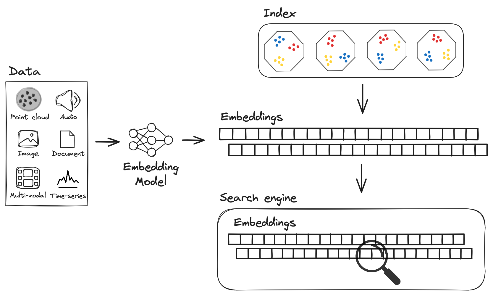
Vector databases store data in a vector format. The input can be anything: text, image, audio, etc. These input will go through embedding model (we will talk about this later). The output of the embedding model is a vector. This vector is stored in the database.
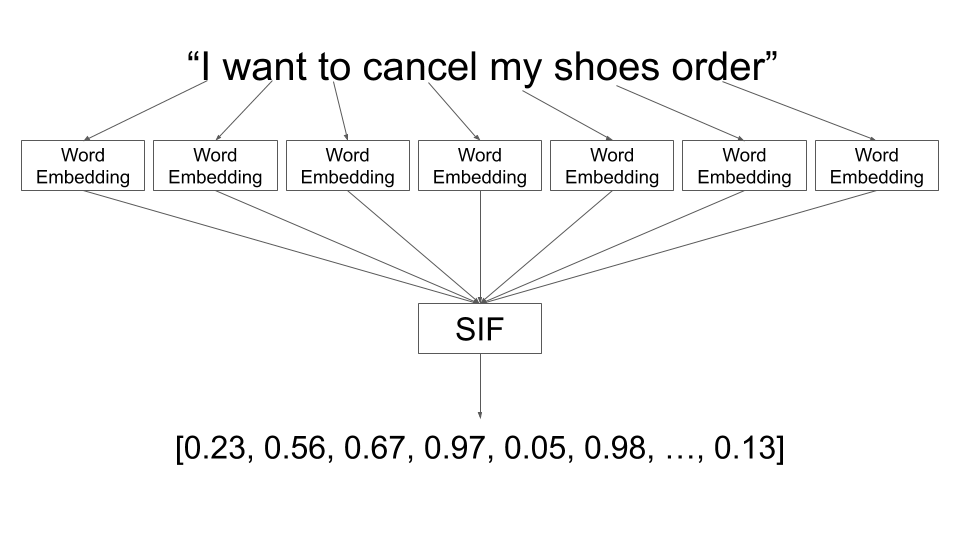 Example of embedding model. Source: engineering.talkdesk.com
When a user make a query (question), the query will go through the embedding model and return as vector. Most vector database will also have similarity search algorithm to find similar vectors data based on the query vector.
In one of the most popular usage of generative AI and vector database is RAG (Retrieval Augmented Generation), vector databses are used to store latest web search results or users’ personal data (PDF, files, etc). You can use RAG to find relevant chunks of text from the database and generate the answer based on the query.
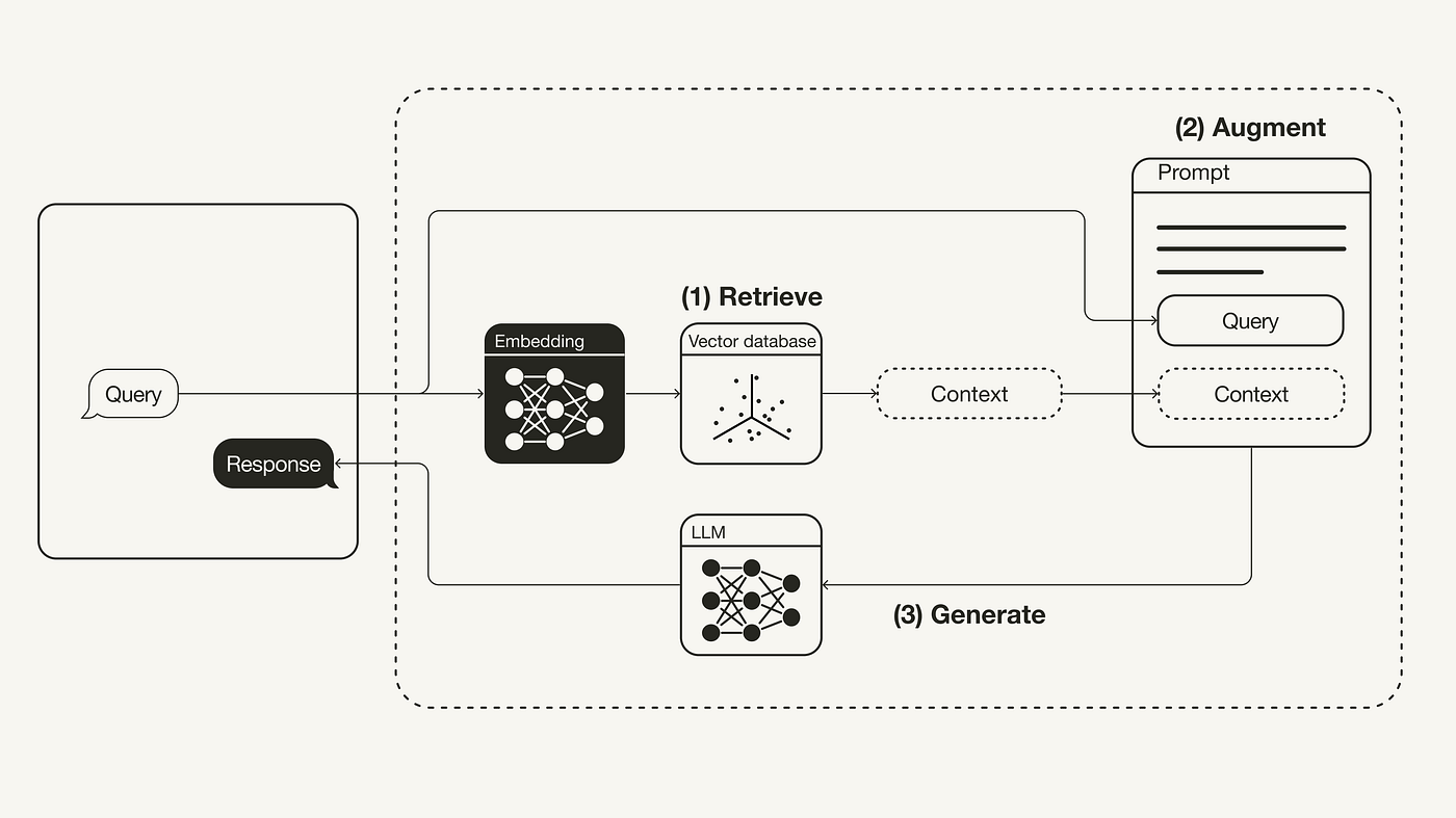 Example of RAG. Source: engineering.talkdesk.com
Similarity search in vector databases
Index
Let’s talk about the secret sauce of vector databases: the vector index. Unlike RDBMS which uses B-tree, or NoSQL with LSM-Tree, vector databases use different kind of index to store and search for similar items.
With NoSQL or SQL, normal database index is a data structure used to improve the speed of data retrieval operations on a database table at the cost of additional space and increased maintenance overhead.
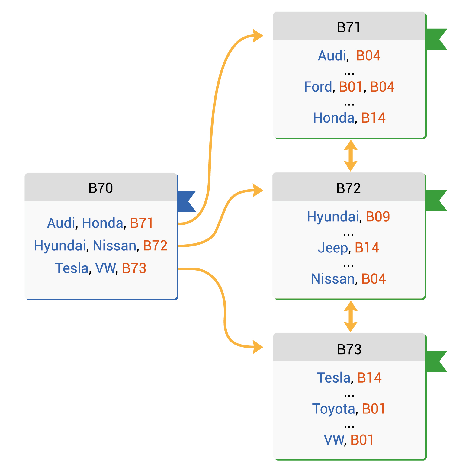 Example of Database index. Source: Vertabelo
In vector databases, the index is used to store the vectors and to search for similar items. There are many types of index, but the most common ones are: FLAT, IVF, SQ, PQ, HNSW, Annoy.
 Example of Vector DB index. Source: LanceDB
We won’t go too much into details since there are already really good blogs and articles about this.
Brute-force search (FLAT)
FLAT is the simplest way to search for similar items. It compares the query vector with all the vectors in the database (O(n)). This is slow and not scalable. However, it is good for small dataset due to being light-weight, especially when parallelized with accelerators like GPUs or FPGAs. Since it loops through all the vectors, it is guaranteed to have the best accuracy. And for flat indexes, that is all we need to do — there is no training (as we have no parameters to optimize when storing vectors without transformations or clustering).
Reason is GPUs are highly parallel processors. FLAT indexing aligns well with this parallel architecture because each vector or data point can be processed independently. This allows for efficient use of GPU resources, as multiple vectors can be indexed or queried in parallel.
Tldr: Good for small dataset, best for accuracy when search speed is not relevant, not scalable and very slow, use for small index (<10K) (will talk about index measurement later).
Currently supported by: Weaviate, Milvus, FAISS.
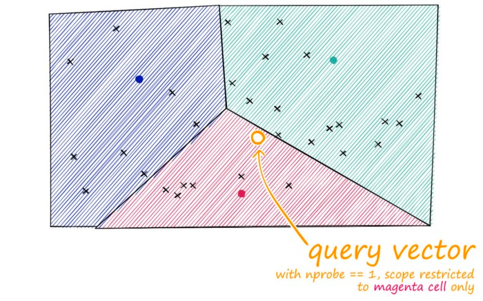
Inverted file index (IVF) - slowest but most accurate
We know that FLAT is most accurate but slow. What is the faster optimization? IVF.
IVF is an indexing method that partitions the database vectors based on their proximity to centroids. These centroids are found through unsupervised clustering, usually k-means. After determining centroids and assignments, we establish an inverted index, linking each centroid to a list of vectors in its cluster. IVF is typically reliable for small to medium datasets.
 IVF. Source: pinecone.io
The reason why it is faster than FLAT is because it uses clustering to group similar vectors together. When a query is made, the search is limited to the cluster that the query vector belongs to. This reduces the number of vectors to compare with.
Other subsets of IVF: IVF_FLAT, IVF_SQ, IVF_PQ (Milvus).
Currently supported by: Milvus; pgvector (IVF_FLAT, IVF_PQ), LanceDB (IVF_PQ).
Tldr: Good scalable option. High-quality, at reasonable speed and memory usage. Good for small to medium dataset.
IVF-Flat indexes use inverted file indexes to rapidly narrow down on the search space, which are much faster than brute force search, but they sacrifice some accuracy in the form of recall
Hierarchical Navigable Small Worlds (HNSW) - most commonly used
IVF is faster than FLAT but what if it is still not fast enough for our use. The next answer is HNSW.
HNSW is the most commonly used vectoring indexing strategy today. It has super fast search speeds and fantastic recall. The main idea of HNSW is to construct such a graph where a path between any pair of vertices could be traversed in a small number of steps. There are 2 foundational concepts you need to know to understand HNSW: Skip lists and Navigable Small World.
Skip list:
 Skip list. Source: Wikipedia
To put it simply, a skip list is a data structure that allows for fast search within an ordered sequence of elements. It is a probabilistic data structure that uses multiple linked lists to skip over elements that are not relevant to the search. It has O(log n) search, delete, and insert time complexity.
Navigable Small World:
Navigable Small World (NSW) models encompass networks with (poly/)logarithmic complexity where greedy routing is utilized. However, the effectiveness of greedy routing diminishes as the network scales up, particularly for larger networks with 1-10K+ vertices, especially when the graph is not navigable [1]. When exploring an NSW graph, we commence from a predetermined entry point which connects to several adjacent vertices. By discerning the closest vertex to our query vector among these connections, we proceed to it. This process iterates through greedy-routing, moving from vertex to vertex by selecting the nearest neighboring vertices within each vertex’s friend list. Eventually, we reach a local minimum where no closer vertices exist, serving as our termination point.
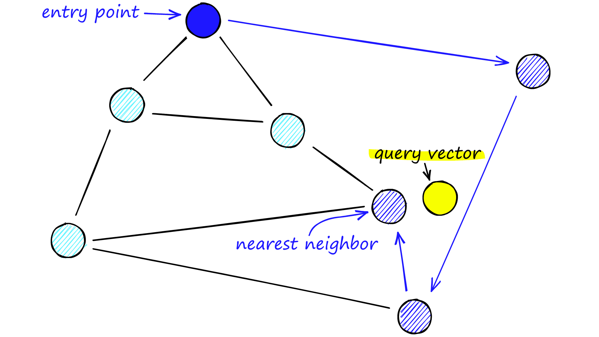 Navigable Small World. Source: pinecone.io
However, NSW graphs are not always navigable, particularly when the graph is large or the data is high-dimensional. To address this, Hierarchical Navigable Small World (HNSW) graphs were introduced. HNSW graphs are navigable and hierarchical, with each level containing a subset of vertices from the previous level. This hierarchical structure allows for faster search times and improved recall.
HNSW:
HNSW is a graph-based index that uses a multi-level graph to store vectors. For each layer, we go through the same process as NSW until we find the closest vertex. The difference is that we store the vertex in the next layer. This process continues until we find the local minimum of our bottom layer — layer 0.
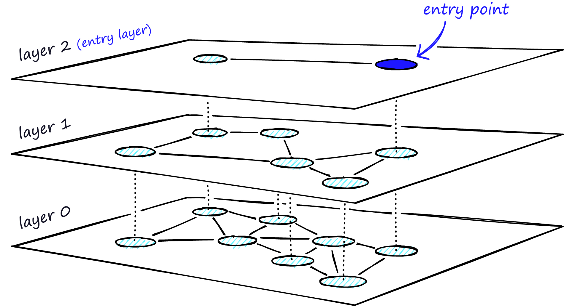 HNSW. Source: pinecone.io
The reason why it is fast is because of ANN (Approximate Nearest Neighbor) search. ANN search is a search algorithm that finds the approximate nearest neighbors of a query vector. It is fast because it focuses on finding approximate nearest neighbors rather than exact matches. However, there is always a trade-off between speed and memory usage. HNSW is fast but uses more memory than IVF due to the complexity of the graph and number of connections of the nodes.
In short, HNSW is:
- Build a hierarchy of layers to speed up the traversal of the nearest neighbor graph.
- In this graph, the top layers contain only long-range edges.
- The deeper the search traverses through the hierarchy, the shorter the distance between vectors captured in the edges.
Tldr: Fastest search speed, high-quality, good for medium to large dataset, comes with higher memory usage.
Product quantization (PQ)
Now, we have come to high memory usage problem. One of the reason is the high-dimensional data.
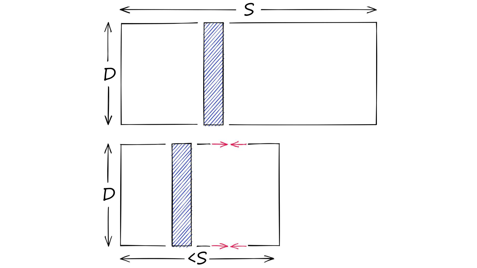
Product quantization (PQ) is a popular method for dramatically compressing high-dimensional vectors to use less memory.
 Product quantization. Source: pinecone.io
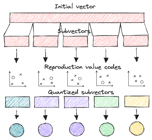
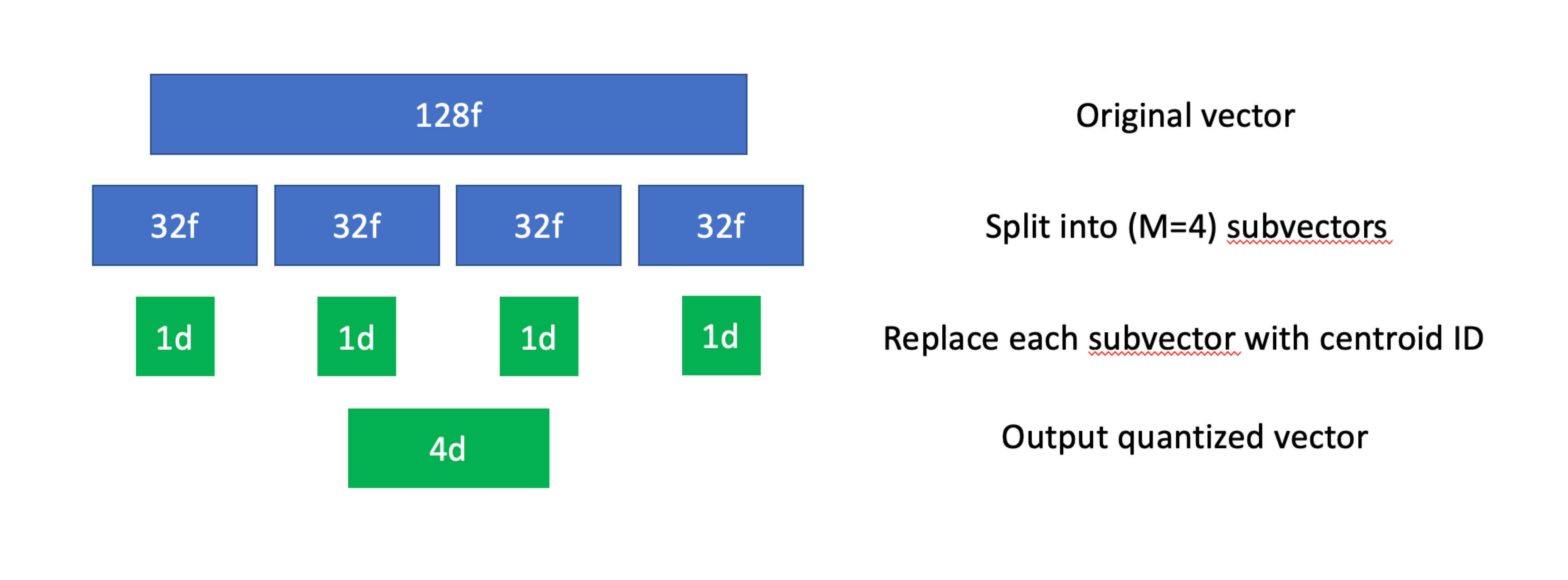
In short, PQ is the process of:
- Taking a big, high-dimensional vector,
- Splitting it into equally sized chunks — our subvectors,
- Assigning each of these subvectors to its nearest centroid (also called reproduction/reconstruction values), usually using k-means clustering.
- Replacing these centroid values with unique IDs — each ID represents a centroid
 Product quantization. Source: thedataquarry.com
However, PQ is not as accurate as FLAT; it has acceptable speed.
Tldr: Lowest memory usage, acceptable speed, less accurate than FLAT.
IVF-PQ uses IVF in combination with Product Quantization to compress the vectors, reducing the memory footprint and speeding up search, while being better in recall than a pure PQ index
Scalar quantization (SQ)
Next we will learn about scalar quantization, which is used in Qdrant.
Scalar quantization converts floating-point vectors (typically float32 or float64) into integer vectors by dividing each dimension into bins. The process involves:
-
Determining the maximum and minimum values of each dimension.
-
Calculating start values and step sizes.
-
Performing quantization by subtracting start values and dividing by step sizes.
The quantized dataset typically uses 8-bit unsigned integers, but lower values (5-bit, 4-bit, and even 2-bit) are also common.
PQ and SQ are similar in that they both compress vectors to reduce memory usage. However, PQ compresses vectors by dividing them into subvectors and assigning each subvector to a centroid, while SQ compresses vectors by dividing them into bins and converting them to integers. They are different methods to achieve the same goal: reducing memory usage.
 Scalar quantization. Source: zilliz.com
Other candidates
Approximate Nearest Neighbors Oh Yeah (Annoy)
Annoy (Approximate Nearest Neighbors Oh Yeah) is an algorithm based on random projections and trees. It is a tree-based index that uses binary search trees as its core data structure. It partitions the vector space recursively to create a binary tree, where each node is split by a hyperplane equidistant from two randomly selected child vectors. The splitting process continues until leaf nodes have fewer than a predefined number of elements. Querying involves iteratively the tree to determine which side of the hyperplane the query vector falls on.
 Annoy idea. Source: sds-aau.github.io
Annoy is fast because it has the ability to use static files as indexes. In particular, this means you can share index across processes. Annoy also decouples creating indexes from loading them, so you can pass around indexes as files and map them into memory quickly. Another nice thing of Annoy is that it tries to minimize memory footprint so the indexes are quite small. The original idea was to sacrifice some accuracy for speed.
Annoy comes with the curse of dimensionality. The curse of dimensionality is a phenomenon that occurs when the number of dimensions in a dataset increases, causing the volume of the space to grow exponentially. This results in the data points becoming increasingly sparse, making it difficult to find meaningful patterns or relationships. Annoy is not suitable for high-dimensional data, as it can lead to poor performance and accuracy. For example, 100M vectors alone will require approximately 400GB of RAM.
It’s not recommended to use Annoy for high-dimensional data, compared to HNSW.
DiskANN
DiskANN is new. DiskANN is on-disk index method that utilizes both RAM and hard disk, which is based on Vamana data structure.
Vamana’s key concept is the relative neighborhood graph (RNG) 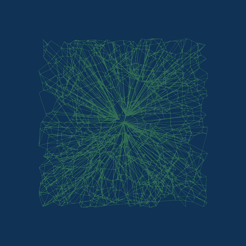 Relative neighborhood graph. Source: Wikepedia.com
In short, Vamana is
- Build a random graph.
- Optimize the graph, so it only connects vectors close to each other.
- Modify the graph by removing some short connections and adding some long-range edges to speed up the traversal of the graph.
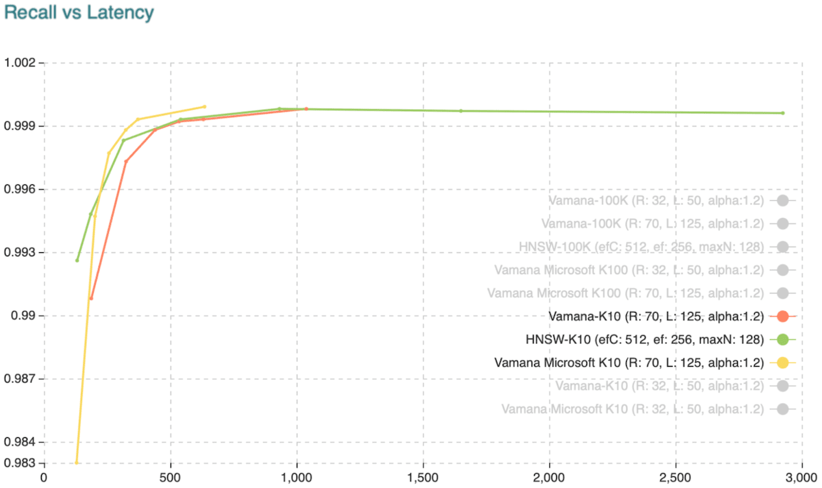 Recall vs. Latency when retrieving the ten approximate nearest neighbors. Source: weaviate.io
DiskANN is slightly faster and more accurate than HNSW. However, there are only 2 implementations of DiskANN: Weaviate and Qdrant in the vector database market.
Similarity metrics
When choosing the optimal similarity metric for your index, a key guideline is to align it with the metric utilized during the training of your embedding model. For instance, since the all-MiniLM-L6-v2 model was trained with cosine similarity, employing cosine similarity for the index will yield the most precise outcome.
The most common similarity metrics are: cosine similarity, Euclidean distance, and Dot product similarity.
We won’t go too much into the mathematics implementations but cosine similarity is the most common one amongs embedding models like GPT-4.
From OpenAI: “OpenAI embeddings are normalized to length 1, which means that:
Cosine similarity can be computed slightly faster using just a dot product Cosine similarity and Euclidean distance will result in the identical rankings”
Read more about different similarity metrics here.
Pick the right vector database
When choosing a vector database, consider the following factors:
- The right database for your engineering need (speed, scalability, etc) which comes to indexing method.
- The cost of the database and possible vendor lock-in.
- The support (community, documentation, etc).
- The limitation.
Engineering needs
So far, we have coverred speed, scalability, accuracy, and memory usage. Let’s put the index methods first into table.
| Index | Speed | Scalability | Accuracy | Memory usage (higher is bad) |
|---|---|---|---|---|
| FLAT | Slow | Not scalable | Very High | High |
| IVF | Medium | Medium | High | Medium |
| SQ | Medium | Medium | Medium | Low |
| PQ | Medium | Medium | Medium | Low |
| HNSW | Fast | High | High | High |
| Annoy | Fast | High | High | High |
| DiskANN | Fast | High | High | Low |
When you are choosing a vector database, it is firstly about index size.
If you want 100% recall, use FLAT.
- index_size < 10MB: Use
FLAT - 10 MB < index_size < 2GB: Use
IVF - 2GB < index_size < 10GB:
- Use
HNSWif you want high recall but high memory usage - Use
PQif you want low memory usage but less accurate - Use IVF_PQ, IVF_SQ if you want have limited compute resources.
- Use
- 20GB < index_size < 200GB: large dataset. use
IVF_PQfor memory-constrained applications andHNSW_SQfor applications that require high recall (same speed as HNSW but reduced index size).
Something more to read on indexing 1M vectors here.
Based on this, let’s put top vector databases with their index method. Things might change in the future. I recommend to check the latest information.
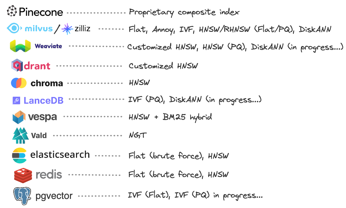 Vector database and their index method. Source: thedataquarry.com
Cost When many services share the same techniques (as businesses, most will find ways to catch up with the competition aka there is no bad method, just use for the right use case), the cost will be the deciding factor. I won’t list the cost here since it is always changing. There is also a competition to make the cost lower or similiar.
However, from my observation, the cost of tools can be lower than the cost of engineers. So, it’s important to choose the tool that most engneers find comfortable with.
More on supprt and limitation, I recommend to check the more on this blog here.
To put it shortly,
| Database | Pros | Cons |
|---|---|---|
| Pinecone | Very easy to get up and running | Fully proprietary |
| Weaviate | Amazing documentation, support Docker | Require infra resources |
| Qdrant | Built in Rust, lower resource utilization | Not as mature as others |
| Milvus/Zilliz | Mature, has DiskANN | Milvus’s system is complex and resource-intensive |
| Chroma | Has embedded mode by default, has Python/JS interface | Does not have storage layer, depends on Clickhouse |
| LanceDB | Built in Rust, support multi-modal data | Not as mature as others |
| Vespa | Most “enterprise-ready” hybrid search capabilities | Application layer written in Java, is not straightforward to tear down development instances, for example via Docker and Kubernetes. |
| Vald | Multi-modal data, index backup, fast ANN search | Less overall traction |
| Elasticsearch, Redis and pgvector | No need to learn new tools due to its popularity | More general-pupose, not as optimized for vector search |
| KDB.AI | Optimized for time series, columnar format data, good for financial data | Not as mature as others |
I strongly recommend reading blog posts by thedataquarry.com. They have put a lot of effort to compare these databases. One of them the use on-prem vs cloud.
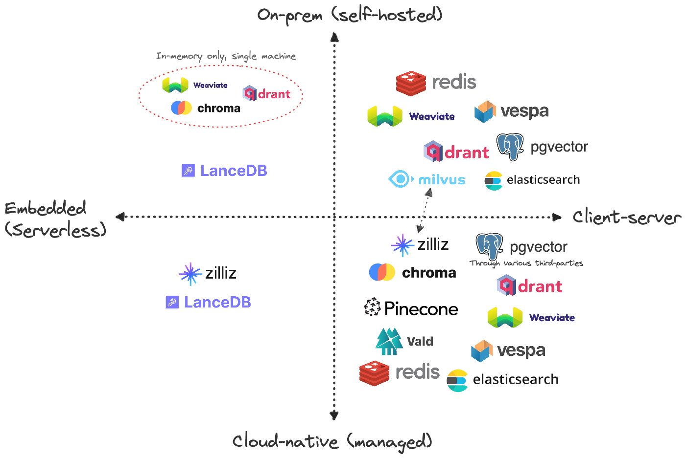 On-prem vs cloud. Source: thedataquarry.com
More on here
Last words
I believe vector database is the future of AI, at least with reccommendation task. For SWEs who want to get involved with AI without changing into data scientist, learning about vector database is a good start since it is more backend focused and data is always important.
There will be a need to upskill of course. Before with normal database, you only need to learn B-Tree, LSM-Tree, etc. Vector database has more indexing method and you need to know which one to use. Some fundamentals in math and statistics are also needed to understand vectors, embeddings, and how these calculations will affect the system, why it is faster or slower. As machine learning is being taught at most colleges, I strongly recommend one to understand deeply how foundational machine learning techniques work (unsupervised learning, graph theory, etc), not just using libraries. One might argue why it is important since cloud providers already implemented these libraries. But understanding the fundamentals will help you to debug, optimize, and scale the system once you get higher levels.
This is how I believe backend developers can get involved with AI without changing their career path.
Terms to know: embeddings, vector, index, k-means, unsperivised learning, skip list, ANN, greedy search, Vanama.
I also created some implementation of the vector database (no wrapper) with Python. You can check it here.
References:
- https://thesequence.substack.com/p/guest-post-choosing-the-right-vector
- https://kdb.ai/learning-hub/articles/indexing-basics/
- https://zilliz.com/learn/vector-index
- https://thedataquarry.com/posts/vector-db-3/
- https://www.sciencedirect.com/topics/computer-science/floating-point-vector
- https://www.pinecone.io/learn/series/faiss/product-quantization/
- https://qdrant.tech/articles/scalar-quantization/
- https://sds-aau.github.io/M3Port19/portfolio/ann/
- https://modelz.ai/blog/pgvector
- [1] M. Boguna et al., Navigability of complex networks (2009), Nature Physics, vol. 5, no. 1, pp. 74-80
Enjoy Reading This Article?
Here are some more articles you might like to read next: